How Does Neural Networks Detect Fake Faces?

 

Introduction:

The detection of fake faces or more generally fake (or photoshopped) images is relatively a simple task for the human eye, and that is because of the amazing ability of the human brain to detect manipulated patterns or patches in the image. So, basically, in case of fake faces detection, the human brain usually looks for the what seems to be manipulated or deformed areas of the image and by comparing that with what certain face features should look like, we can naturally make a prediction whether the image is of a fake or real face. However, there are cases where we can not make a certain decision, especially if the deformed features are on pixel level size or if the AI generated face checks all the normal face features for the human eyes, such as the last face image in the below. The figure below shows 6 fake faces with different degrees of difficulty to detect them.

Convolutional neural networks have proven their robustness and efficiency in many computer vision problems, more particularly in image classification. So, we can train a convolutional neural network to classify fake and real faces with a very high accuracy score. However, what intrigued me most while training such network, is to discover how does such a neural network detect the fake face images? And more precisely, does the neural network detect the fake patterns and assign to them higher degree of pertinence when producing the prediction or not?

So, to answer this question, I discovered a whole new area in the AI domain, which is Explainable AI. Fundamentally, Explainable AI aims for discovering why an AI arrived at a specific decision. In Computer Vision, many techniques have been developed to allow us to take a look on the behavior of convolutional neural networks and to understand how they produce predictions.

Beside the understandability aspect, being able to translate calculations made by a neural network into visuals that can be understood by humans, helps us improve the performance of the model and avoid issues like; Age, sex, and ethnicity biases.

Some of the techniques that are developed for Computer Vision models interpretations are the following:

1. SHAP or SHapley Additive exPlanations: It is described by its developer as follows “SHAP is a game theoretic approach to explain the output of any machine learning model. It connects optimal credit allocation with local explanations using the classic Shapley values from game theory and their related extensions.” Basically, the open source SHAP package provides tools that can be used with any simple or complex machine learning model to understand which features are most important for the model. SHAP can also be used with different types of models such as; Linear Regression, Logistic Regression, Gradient Boosting, SVMs, and Neural Networks. In computer vision, SHAP can also be used to visualize which part of the image are most important for a given prediction.
2. Feature Maps: feature maps are used to visualize what a model is “seeing” through a set of convolutional filters. It makes it possible for us to understand how the learned filters are making the model recognizing a certain class. The implementation of this method is straightforward and can be don’t using any deep learning framework.
3. Occlusion Sensitivity: It is another simple technique for understanding which parts of an image are most important for a deep network's classification. This method is used to visualize how parts of the image affects neural network's confidence by occluding parts iteratively.
4. Grad-CAM or Gradient-weighted Class Activation Mapping: This method was introduced in 2016 by Ramprasaath R. Selvaraju et al. where they propose a technique for producing "visual explanations" for decisions from a large class of CNN-based models. Given an input image, this method is used to compute a heatmap for any convolutional layer of a CNN model. The heatmap represent the areas that the model mostly focused on when producing the predicted class.

In the present article, I’ve chosen to utilize the Grad-CAM algorithm to try to answer the question we posed, and that is because of the simplicity of the implementation of the algorithm as well as its well-known good performance in many research papers.

Therefore, we will train a CNN model using a ResNet architecture to classify real and fake face images, then we’re going to use Grad-CAM and Guided Grad-CAM to visualize, which part of the input image was the model focusing on for the given class prediction. But before discussing the training process let’s take a quick look on the Grad-Cam algorithm.

Grad-CAM Algorithm:

The Gradient-weighted Class Activation Mapping algorithm can be implemented in two phases; As portrayed in the figure below, the first phase consists in performing forward propagation and saving both the output of the model (Class prediction), and the output of the Convolutional layer, which is also known as the feature activation map.

In the second phase, as shown in the figure below, we can calculate the Grad-CAM heatmap following 3 steps:

1. Calculating the derivatives of the predicted class with respect to the chosen feature activation map via backprop.
2. Calculating the neuron importance weights by taking the global-average-pooling of the derivatives calculated in the previous step.
3. Calculating the linear combination of the produced neuron importance weights and the feature activation map, then applying the ReLU function on the resulted tensor.

The result is then a heatmap that can be resized and displayed over the input image to visualize the most activated regions of the image for the class that’s been predicted.

As you may have noticed in the Grad-CAM algorithm illustration, there is a part that we haven’t discussed yet and it is about the Guided Grad-CAM, but you don’t need to worry about it for now, we’re going to discuss it later on in this article.

The results of any deep learning application depend heavily on the model architecture as well as on the data, so preparing a “good” dataset which meets a certain number of criteria is crucial to obtain the desired results.

Datasets & Training:

Datasets:

In this project, I have used 2 public datasets available on Kaggle. The first one contains 140k face images split evenly between both classes, and it represent 100% of the training data. And I created the second dataset using Unsplash API to gather real face images and the StyleGan2 to collect the fake faces images. My goal was to create a Test set for my model that is challenging enough even for human beings. The dataset I created is also publicly available on Kaggle.

Training process:

The training process was conducted following a standard fine-tuning strategy, where the training dataset which consists of 40k images, is  preprocessed and then used to train the new head of a pretrained ResNet model along with the last convolutional layer of the ResNet. 

The model is trained for 20 epochs using the Adam optimization algorithm with an early-stopping and LR-reducer callbacks.

Results:

The trained model is then used to perform Grad-CAM and Guided Grad-CAM on a sample of images. But, we need first to know what is exactly the Guided Grad-CAM?

Guided Grad-CAM:

To put it in simple and few words, the Guided Grad-CAM is simply a combination of Grad-CAM and Guided backpropagation. Where guided backpropagation is a technique used to visualize which pixels of an image are activating the neurons of a certain layer during the performance of backpropagation, and that is done by utilizing a guided ReLU function instead of the regular ReLU.

Thus, The pixels that are not activating any neurons or that are having negative activations are neglected (gray pixels in resulted image).

Now, let's discuss the results obtained by our trained model. You can use this notebook on Kaggle to reproduce or check more results. 

let’s find out how does a neural network detect fake faces!

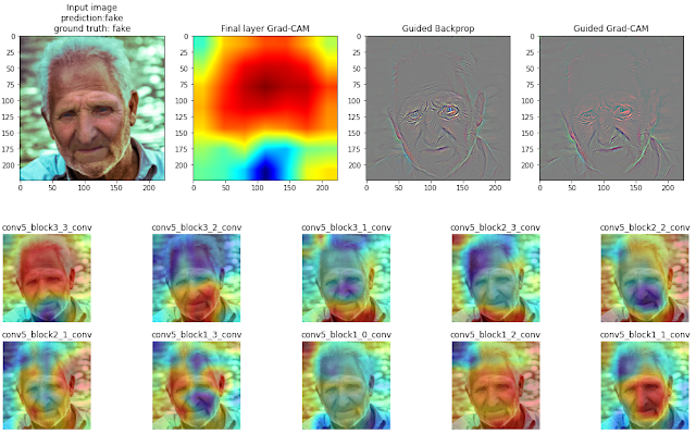
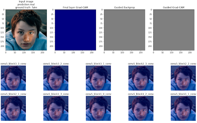
The results will be presented using some images as examples, with different levels of difficulties to the human eyes. The Grad-CAM heatmap is calculated and displayed for the last 10 convolutional layer of the model, whereas the guided backprop and guided Grad-CAM are only shown for the last convolutional layer of the model, which is the one that was fine tuned.

The model reached 0.85 average F1-score on the test set, so we’re going to look for both positive and negative examples and discuss each case further.

Obviously altered images:

This first image is a fake face image, that is easily detected by the human eyes, we can clearly see that the eyes and nose parts where manipulated. The Grad-CAM results on the last layer shows that the model is focusing on the upper region of the face with more emphasis on the boundary between the real part and manipulated part of the face. 

Given that the model has correctly classified this image as fake, we can say that it has came to that conclusion in s similar way as a human eye would do, which is by focusing on the odd part of this mage.

Furthermore, we can see that in the guided backprop and Guided Grad-CAM, the pixels that has activated the convolutional layers the most are around the eyes region of the face, this can further confirm that the pixels that are on the manipulated part are the ones that are mostly activating the neurons to produce the correct prediction.

More images that shows similar behavior as for the first one are displayed below:

Even though the model predicts correctly the fake images that present altered eyes regions, many other images shows that the model fails to detect the manipulation of other regions of the face such as the nose, mouth, or ears regions. The following image shows that the model fails to predict a fake image which exhibit a manipulation of the nose and left-eye regions.

As shown above, the Grad-CAM heatmap is all blue and that is understandable since the model predicts that this is a real image, therefore no region is contributing to the "fake" label.

Another example of  mislabeling an "easy" image:

Based on these first results, we can suggest that we need more images containing different types of manipulated areas other that the eyes region to train the model to remedy this issue.

Hardly detected altered images:

In this second case, we're investigation the model performance on images that are harder to detect as fake by the human eyes. For instance the first as much as I tried to detect the issue with the example shown above, I couldn't come to the conclusion that it is a manipulated image. However, we can see that the model correctly labeled the image. 

Moreover, the Grad-CAM and Guided Grad-CAM results informs us that the model focused mainly on the upper region of the face with more focus on the ear region. Even though we can't see what's wrong with those regions, we can conclude that on a pixel level, the model has detected some issues with that region of the face image.

another case where manipulated images are hard to detect is when the manipulated area is not part of the face. As shown in the image above, the model correctly classified the image, and we can see that the model was focusing more on the hair region surrounding the face. 

Even though it's hard to label this image by the human eye, the model suggest that the hair part was altered and if we zoom in of the image we can see some odd behavior on the extremity of  hair which blend in with the background, see image below.

In other cases, the model fails to correctly label images such as in the image below, It clearly shows a real face image, however the model thinks that it is a fake face and it even shows that the model focused more on the face rather that the background, which is a repeated behavior that I remarked for this model and in some cases it lead to mislabeling easier images.

The image below shows that sometimes the model focuses on the wrong regions of the image, which is a problem that should be addressed to better the performance of the model.

Real images:

In this last paragraph, we're going to discuss the performance of the model on real images. The images below shows the results on a sample of real images.

The model shows similar results on the majority of the images that were correctly labeled as "real", i.e. with no neuron activation for the "fake" label. Although, in some cases where the model prediction was made with low confidence, we can visualize some activations that led to the lack of confidence for the prediction, as shown in the images below.

Conclusion:

We’ve seen that using Grad-CAM we can investigate the model behavior and have a clear view on how it came to the predication that was made. Grad-CAM provided us with a visual way of  testing the performance of a model, and by discussing the results of a sample of images, we can take notes on what the model fails to do and what it is more inclined towards when performing a prediction. Based on the remarks that we made, we can then make the right adjustments to increase the performance of the model.

In this case of fake face detection, we’ve seen that the model was able to behaved like human in some ways. The model successfully managed to focus on the face features in many cases, but it has failed to produce the correct results in others. One way to improve this model performance is to use more images of fake faces that includes, small distortions or manipulation of some areas of the face, and face images with fake backgrounds to make the model pay more attentions to smaller details on the face and to the image backgrounds with can be a great indicator of image manipulation.

The work is done on Kaggle, and a public notebook is available via this link.